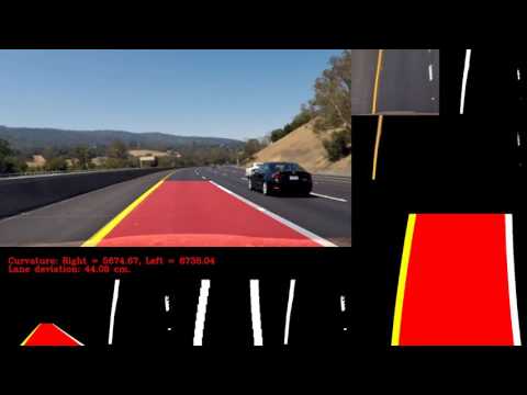
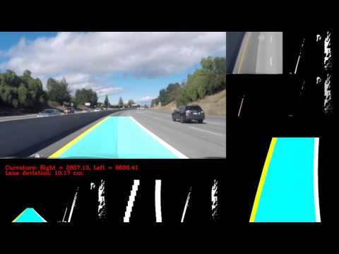
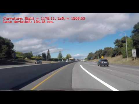
Lane finding is crucial for developing algorithms for autonomous driving robots or self-driving cars. The lane-finding algorithm must be robust to changing light conditions, weather conditions, other cars/vehicles on the road, curvature of road and type of road itself. In this post, we present an algorithm based on advanced computer vision techniques to identify left and right lanes from dash-mounted camera video. This is second submission for the Advanced lane finding project of Udacity's Self-driving car nanodegree. The objective in this project was to apply advanced computer vision techniques to detect lanes and locate the car between the two lanes and compute curvature of the road. The final outcome is illustrated in the figure below.
In the notebook below, we will go over the steps taken to go from the image in the left panel to the image in the right panel.
The algorithm is divided into two steps, in the first step we apply a perspective transform and compute a lane mask to identify potential locations of lane in an image, and in the next step we combine the lane mask information with previous frame information to compute the final lane. The second step is performed to discard effects of noisy or
Figure below presents the steps involved in obtaining lane masks from the original image. The steps are divided as follows,
- Read and undistort image: In this step, a new image is read by the program and the image is undistorted using precomputed camera distortion matrices.
- Perspective transform: Read in new image and apply perspective transform. Perspective transformation gives us bird's eye view of the road, this makes further processing easier as any irrelevant information about background is removed from the warped image.
- Color Masks: Once we obtain the perspective transform, we next apply color masks to identify yellow and white pixels in the image. Color masks are applied after converting the image from RGB to HSV space. HSV space is more suited for identifying colors as it segements the colors into the color them selves (Hue), the ammount of color (Saturation) and brightness (Value). We identify yellow color as the pixels whose HSV-transformed intensities are between \([ 0, 100, 100]\) and \([ 50, 255, 255]\), and white color as the pixels with intensities between \( [20, 0, 180]\) and \([255, 80, 255] \).
- Sobel Filters: In addition to the color masks, we apply sobel filters to detect edges. We apply sobel filters on L and S channels of image, as these were found to be robust to color and lighting variations. After multiple trial and error, we decided to use the magnitude of gradient along x- and y- directions with thresholds of 50 to 200 as good candidates to identify the edges.
- Combine sobel and color masks: In a final step we combined candidate lane pixels from Sobel filters and color masks to obtain potential lane regions.
These steps are illustrated in the figure below.
From above, we get good representation of lane masks. However, these masks are based on yellow and white colors and sobel filter calculations. If there are additional drawings or markings on the road, this algorithm will not give two neat lines as above, we will therefore perform additional analysis to isolate the lane loactions.
We implement different lane calculations for the first frame and subsequent frames. In the first frame, we compute the lanes using computer vision methods, however, in the later frames, we skip these steps. Instead, we place windows of 50 pixel width centered on the lanes computed in the previous frame, and search within these windows. This significanly reduced the computation time, for our algorithm. We were able to achieve 10 Frames/s lane estimation rate.
The next step is to compute lanes for the first image. To do so, we take the lane mask from the previous step, and take only the bottom half of the image. We next use scipy to compute the locations of the peaks corresponding to the left and right lanes.
We then place a window of size 50 pixels centered at these peaks, and search for peaks in the bottom 8th of the image. Next we move up to the next 1/8th of the image and center windows at the peaks detected in the bottom 1/8th of the image. We repeat this process 8 times to cover the entire image. This is illustrated in the figure below.
In addition to tracking the location of the previous window, we also keep track of the displacement of previous window. In cases where no peaks are found, we place a window centered at the location calculated assuming the location of previous window moved by a precomputed offset. The windows and lanes obtained after this step are shown below.
We next fit a quadratic function with independent variable 'x' and dependent variable 'y' to the points within the line mask using numpy's polyfit function.
After computing the lanes, we draw them back on the original undistorted image as follows.
If the current frame is not the first frame, we follow the same steps as part 2 to get the lane masks, however, we introduced additional steps to ensure any error due to incorrectly detected lanes is removed. Lane correction are introduced as,
- Outlier removal 1: If the change in coefficient is above 0.005, the lanes are discarded. This number was obtained empirically.
- Outlier removal 2: If any lane was found with less than 5 pixels, we use the previous line fit coefficients as the coefficients for the current one.
- Smoothing: We smooth the value of the current lane using a first order filter response, as \(coeffs = 0.95*coeff~prev+ 0.05 coeff\).
Finally , we use the coefficients of polynomial fit to compute curvatures of the lane, and relative location of the car in the lane.
Videos below show performance of our algorithm on project and challenge videos.
This was a very tedious project involving tuning of several parameters. This project let me to appreciate deep learning based approaches even more. Computer vision solutions are sensitive to the chosen parameters, and if the parameters are not chosen correctly, they fail. Deep learning approaches avoid the need for fine-tuning these parameters, and are inherently more robust. I couldn’t get the approach to work on the harder-challenge video, mainly because the lanes had large curvature, and as a result the lanes went outside the region of interest we chose for perspective transform. In coming weeks, I will work on improving performance of the model on the harder challenge video.


