RLP_trees_and_EthStorage.md

Recursive Length Prefix (RPL) Encoding

RLP is an encoding/decoding algorithm that helps ethereum to serialize data and make possible to reconstruct it quickly.

RLP encoding:

1. If input is a single byte between the [0x00 and 0x7F] range it's RLP encoding it's itself.

2. If the input is non-value (Uint(0), []byte{}, string"", empty pointer..) RLP encoding is 0x80. Notice that 0x00 value byte is not non-value.

3. If input is a special byte between [0x80, 0xFF] range, RLP encoding will concatenate 0x81 with the byte: [0x81, the_byte]. Example: RLP_encode(0x80)(a byte that represents something on ASCII) = [0x81, 0x80].

4. If input is a string with 2–55 bytes long, RLP encoding consists of a single byte with value 0x80 plus the length of the string in bytes and then array of hex value of string.

For Example: "hello world" = [0x8b, 0x68, 0x65, 0x6c, 0x6c, 0x6f, 0x20, 0x77, 0x6f, 0x72, 0x6c, 0x64]
Because "hello world" has 11 bytes in hex (0x0b in hex) the first byte of RLP encoding is:
0x80 + 0x0b = 0x8b , after that we concatenate the bytes of "hello world".

5. If input is a string with more than 55 bytes long, RLP encoding consists of 3 parts from the left to the right.
   • The first part is a single byte with value 0xb7 plus the length in bytes of the second part. - The second part is hex value of the length of the string.
   • The last one is the string in bytes. The range of the first byte is [0xb8, 0xbf].

For example: a string with 1024 “a” characters, so the encoding is “aaa…” = [0xb9, 0x04, 0x00, 0x61, 0x61, …]. 

As we can see, from the forth element of array 0x61 to the end is the string in bytes and this is the third part. The second part is 0x04, 0x00 and it is the length of the string 0x0400 = 1024. The first part is 0xb9 = 0xb7 + 0x02 with 0x02 being the length of the second part.

6. If the input is an Empty Array, it's RLP encoding it's a single byte: 0xc0.
7. If the input is a list with total payload in 0–55 bytes long, RLP encoding consists of:
   • A single byte with value 0xc0 plus the length of the list.
   • Then the concatenation of RLP encodings of the items in list. The range of the first byte is [0xc1, 0xf7].

For example: [“hello”, “world”] = [0xcc, 0x85, 0x68, 0x65, 0x6c, 0x6c, 0x6f, 0x85, 0x77, 0x6f, 0x72, 0x6c, 0x64]. In this RLP encoding:

[0x85, 0x68, 0x65, 0x6c, 0x6c, 0x6f] is RLP encoding of “hello”. [0x85, 0x77, 0x6f, 0x72, 0x6c, 0x64] is RLP encoding of “world”. 0xcc = 0xc0 + 0x0c with 0x0c = 0x06 + 0x06 being the length of total payload.

8. If input is a list with total payload more than 55 bytes long, RLP encoding includes 3 parts.
   • The first one is a single byte with value 0xf7 + the length in bytes of the second part. - The second part is the length of total payload.
   • The last part is the concatenation of RLP encodings of the items in list. The range of the first byte is [0xf8, 0xff].
9. With boolean type, true = 0x01 and false = 0x80 (like empty/null variables).

Ethereum wiki encoding examples:

• The string "dog" = [ 0x83, 'd', 'o', 'g' ]

• The list [ "cat", "dog" ] = [ 0xc8, 0x83, 'c', 'a', 't', 0x83, 'd', 'o', 'g' ]

  • 0xc0(list identifier) + 0x08 (length of the list) = 0xc8.
  • 0x83 = 0x80(String identifier) + 0x03(length of the strig in bytes)

• The empty string ('null') = [ 0x80 ]

• The empty list = [ 0xc0 ]

• The integer 0 = [ 0x80 ]

• The encoded integer 0 ('\x00') = [ 0x00 ]

• The encoded integer 15 ('\x0f') = [ 0x0f ]

• The encoded integer 1024 ('\x04\x00') = [ 0x82, 0x04, 0x00 ]

• The set theoretical representation of three, [ [], [[]], [ [], [[]] ] ] = [ 0xc7, 0xc0, 0xc1, 0xc0, 0xc3, 0xc0, 0xc1, 0xc0 ]

• The string "Lorem ipsum dolor sit amet, consectetur adipisicing elit" = [ 0xb8, 0x38, 'L', 'o', 'r', 'e', 'm', ' ', ... , 'e', 'l', 'i', 't' ]

  • 0xb8 = 0xb7 + 0x01(length of the arraly length bytes).
  • 0x38 = Number of bytes of the string.

RLP deencoding:

According to rules and process of RLP encoding, the input of RLP decode shall be regarded as array of binary data, the process is as follows:

1. According to the first byte(i.e. prefix) of input data, and decoding the data type, the length of the actual data and offset;

2. According to type and offset of data, decode data correspondingly;

3. Continue to decode the rest of the input;

Among them, the rules of decoding data types and offset is as follows:

1. The data is a string if the range of the first byte(prefix) is on the range [0x00, 0x7f] and the string is the first byte itself exactly (it's a char basically, a string of length 1).

2. The data is a string if the range of the first byte is [0x80, 0xb7], and the string whose length is equal to the first byte minus0x80 follows the first byte;

3. The data is a string if the range of the first byte is [0xb8, 0xbf], and the length of the string whose length in bytes is equal to the first byte minus 0xb7 follows the first byte. The string follows the length of the next byte that isn't part of the String length description.

4. The data is a list if the range of the first byte is [0xc0, 0xf7], and the concatenation of the RLP encodings of all items of the list which the total payload is equal to the first byte minus 0xc0 follows the first byte.

5. The data is a list if the range of the first byte is [0xf8, 0xff], and the total payload of the list whose length is equal to the first byte minus 0xf7 follows the first byte. The same sort of situation as the String with more than 1 byte of str length.

What would we do when the length of data is out of range of prefix?

We add more dynamic prefixes after the first byte to represent the length of data. For example, with the [0x80, 0xbf] range of string type, according to the strategy we have done above, we divide this range into halves, one ([0x80, 0xb7]) for string with length in range and one ([0xb8, 0xbf]) for string with the length out of range. The same goes with list.

Prelude to tries.

Compact (Hex-prefix) encoding.

Ethereum still has another encoding called Compact encoding or Hex-prefix (HP) encoding.

Terminologies and tries on Ethereum great HP/trie encoding example:

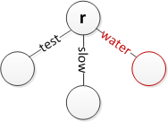
Given a map and a path, find the animal.

Map:

Root: {1: 'Dog', 2: B, 3: A}
A: {1: C, 2: D, 3: 'Cat'}
B: {1: 'Goat', 2: 'Bear', 3: 'Rat'}
C: {1: 'Eagle', 2: 'Parrot', 3: E}
D: {1: 'Shark', 2: 'Dolphin', 3: 'Whale'}
E: {1: 'Duck', 2: 'Chinken', 3: 'Pig'}

Path: 3-2-3.

1. At Root and the first element in path is 3, it means we must get the element of Root which labeled by number 3 and we can see that the value of that element is A.
2. Find node A, the next element in path is 2 so we get the value in node A is D.
3. Find node D, the last element in path is 3, obviously the value we find out is ‘Whale’.

So, the animal of the game is whale.

• Let’s try another path: 3–1–3–2 (the result is ‘Chicken’).

By this, we get familiar with some terminologies:

• Key: Root, A, B, C, D and E will be keys
• Node: Te content corresponding with the key in the right part of each row. For example: {1: ‘Dog’, 2: B, 3: A}.
• Path: The way to be able to derive the trie and find a value. 2–2–3 in example.
• Value: Every element is a key-value pair. Value is the right part of element, value can be a key or a name of animal.
• Nibble: hex form of 4 bits is a nibble. For example: 0x1, 0x4, 0xf …

---

RLP is used for encoding/decoding Value and HP encoding is used for encoding/decoding Path.

HP encoding goals

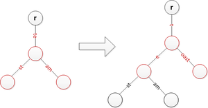
• There are 2 more terminologies which are leaf and extension. Leaf and extension are 2 kinds of node, however path of leaf has terminator and extension does not.

• Terminator is the last byte of the path and has value of 16 in dec or 0x10 in hex.

• It’s possible for a path to have odd length. But odd length is not friendly to turing-machines(Preguntar porqué) and the EVM is one. So we have to convert all odd-length paths to even-length paths. And this is one of the goals oh HP encoding.

In summary, HP encoding goals are:

1. Distinguish leaf and extension from each other without terminator.
2. Convert the path to even length if it's necessary.

HP encoding specification

For now, we call the path inputed in HP encoding as input for convenience.

• If input has terminator, remove terminator from input.
• Create the prefix into input which has value as following table:

node type	path length	prefix	hexchar
extension	even	0000	0x0
extension	odd	0001	0x1
leaf	even	0010	0x2
leaf	odd	0011	0x3

• If the prefix is 0x0 or 0x2 , add a padding nibble 0 next the prefix, so the prefix will be like: 0x00 and 0x20. The main reason to do that is we are trying to maintain the even-length attribute of the path.

• Add prefix to the path

Example of HP encoding:

> [ 1, 2, 3, 4, 5]

'11 23 45'

> [ 0, 1, 2, 3, 4, 5]

'00 01 23 45'

> [ 0, f, 1, c, b, 8, 16]

'20 0f 1c b8'

> [ f, 1, c, b, 8, 16]

'3f 1c b8'

Radix and Merkle tries.

Trie is a word or a terminology that represents digital tree in science computer. Sometime, we can see that ‘tree’ is used, it’s ok because of the same meaning.

In others word, trie is an ordered data structure that is used to store a dynamic set or associative array which is formed to key-value where the keys are usually strings.

Good example to see the different parts of a Trie data structure and to figure out "how it looks like for us".

Radix trie

In computer science, a radix tree (also radix trie or compact prefix tree) is a data structure that represents a space-optimized trie (prefix tree) in which each node that is the only child is merged with its parent.

• The result is that the number of children of every internal node is at most the radix r of the radix tree, where r is a positive integer and a power x of 2, having x ≥ 1. Unlike in regular tries, edges can be labeled with sequences of elements as well as single elements.

• This makes radix trees much more efficient for small sets (especially if the strings are long) and for sets of strings that share long prefixes.

• When r is an integer power of 2 greater or equal to 4, then the radix trie is an r-ary trie, which lessens the depth of the radix trie at the expense of potential sparseness.

Operations

Radix trees support insertion, deletion, and searching operations.

• Insertion adds a new string to the trie while trying to minimize the amount of data stored. - Deletion removes a string from the trie.
• Searching operations include (but are not necessarily limited to): exact lookup, find predecessor, find successor, and find all strings with a prefix. All of these operations are O(k) where k is the maximum length of all strings in the set, where length is measured in the quantity of bits equal to the radix of the radix trie.

LookUp

The lookup operation determines if a string exists in a trie. Most operations modify this approach in some way to handle their specific tasks. For instance, the node where a string terminates may be of importance. This operation is similar to tries except that some edges consume multiple elements.

This will be the representation of the lookup process on a Radix trie:

Insertion

To insert a string, we search the tree until we can make no further progress. At this point we either add a new outgoing edge labeled with all remaining elements in the input string, or if there is already an outgoing edge sharing a prefix with the remaining input string, we split it into two edges (the first labeled with the common prefix) and proceed. This splitting step ensures that no node has more children than there are possible string elements.

Some examples of insertion are:

Root Insertion:

Prefix insertion:

Parent slicing while splitting:

Splitting with deleveling movements

Deletion

To delete a string x from a tree, we first locate the leaf representing x. Then, assuming x exists, we remove the corresponding leaf node. If the parent of our leaf node has only one other child, then that child's incoming label is appended to the parent's incoming label and the child is removed.

Note how the deletion process is done in order to compact data and save space.

Additional searching operations

• Find all strings with common prefix: Returns an array of strings that begin with the same prefix.
• Find predecessor: Locates the largest string less than a given string, by lexicographic order.
• Find successor: Locates the smallest string greater than a given string, by lexicographic order.

Merkle trie

In cryptography and computer science, a hash tree or Merkle tree is a tree in which every leaf node is labelled with the hash of a data block and every non-leaf node is labelled with the cryptographic hash of the labels of its child nodes. Hash trees allow efficient and secure verification of the contents of large data structures. Hash trees are a generalization of hash lists and hash chains.

Demonstrating that a leaf node is a part of a given binary hash tree requires computing a number of hashes proportional to the logarithm of the number of leaf nodes of the tree. This contrasts with hash lists, where the number is proportional to the number of leaf nodes itself.

Hash trees can be used to verify any kind of data stored, handled and transferred in and between computers. They can help ensure that data blocks received from other peers in a peer-to-peer network are received undamaged and unaltered, and even to check that the other peers do not lie and send fake blocks.

Here we have an example.

Note on the example avobe that If L1 changes, it's hash will change, and this will make change the whole path to the root. So it's the perfect way to validate the correctness of any type of data (large ammounts of data also, by using hash functions, the length of the input data doesn't matter).

Proving inclusion

The root of this tree is just a hash — it tells us nothing about the contents of the tree. We can use something called a “Merkle proof” to show that some content is actually part of this tree. For example, let’s prove that A is part of the above tree. All we need to do is provide each of A’s siblings on the way up, recompute the tree, and make sure everything matches. Note that siblings are highlighted in blue.

With just A, H(B), and H(H(C)+H(D)), we can recompute the original root hash. This is an efficient way to show that A is part of this tree without having to provide the entire tree.

Proving Non-inclusion

So we can easily prove that something is part of the Merkle tree, but what if we want to prove that something isn’t part of the tree? Unfortunately, standard Merkle trees don’t give us any good way to do this. We could reveal the entire contents, but that’s sort of defeating the point of using a Merkle tree in the first place.

##Sparse Merkle Trie Here’s where sparse Merkle trees come into play. A sparse Merkle tree is like a standard Merkle tree, except the contained data is indexed, and each datapoint is placed at the leaf that corresponds to that datapoint’s index.

As said by Vitalik here:

A sparse Merkle tree (SMT) is a data structure useful for storing a key/value map which works as follows. An empty SMT is simply a Merkle tree with 2256 leaves, where every leaf is a zero value. Because every element at the second level of the tree is the same (z2=hash(0,0)), and every element at the third level is the same (z3=hash(z2,z2)) and so forth this can be trivially computed in 256 hashes.

Let’s say we have a Merkle tree with four leaves. We’ll populate this tree with some letters (A, D) to demonstrate. The letter A is the first letter of the alphabet, so we should put it at the first leaf. Similarly, we can put D at the fourth leaf.

So what happens in the second and third leaves? We just leave them empty. More precisely, we put a special value (like null) instead of placing a letter.

The tree ends up looking like this:

Provin Inclusion stills being the same as it was before as we can see here: Again, we’re just providing the siblings, H(null) and H(H(null)+H(D)), and checking that it matches the root.

Proving Non-inclusion

Here’s where the magic happens. What happens if we want to prove that C is not part of this Merkle tree? It’s easy! We know that if C were part of the tree, it would be at the third leaf. If C isn’t part of the tree, then the third leaf must be null.

All we need is a standard Merkle proof showing the third leaf is null This looks just like a standard Merkle proof, except that we’re proving the leaf contains null instead of C.

Drawbacks

Sparse Merkle trees are really cool because they give us efficient proofs of non-inclusion. However, this can also mean they get really, really big. 26 letters isn’t much, but most of the time we’re talking about 2²⁵⁶ hashes, which is a large ammount of data.

Luckily, there are some techniques to efficiently generate Merkle trees. The key to these techniques is that these giant sparse Merkle trees are mostly… sparse. H(null) is a constant value, and so is H(H(null)), etc. etc. Huge chunks of the tree can be cached.

Patricia Trie.

Patricia trie is the main trie used in Ethereum to store data. It is a mixture of Radix trie and Merkle trie.

The PATRICIA tree was created in 1968 by Donald R. Morrison, who coined the acronym based on an algorithm he created for retrieving information efficiently from tries; PATRICIA stands for “Practical Algorithm To Retrieve Information Coded In Alphanumeric”.

Merkle Patricia tries provide a cryptographically authenticated data structure that can be used to store all (key, value) bindings. They are fully deterministic, meaning that a Patricia trie with the same (key,value) bindings is guaranteed to be exactly the same down to the last byte and therefore have the same root hash, provide the holy grail of O(log(n)) efficiency for inserts, lookups and deletes, and are much easier to understand and code than more complex comparison-based alternatives.

The most important thing to remember about a PATRICIA tree is that its radix is 2. Since we know that the way that keys are compared happens r bits at a time, where 2 to the power of r is the radix of the tree, we can use this math to figure out how a PATRICIA tree reads a key.

Since the radix of a PATRICIA tree is 2, we know that r must be equal to 1, since 2¹ = 2. Thus, a PATRICIA tree processes its keys one bit at a time.

Because of this, each node in a PATRICIA tree has a 2-way branch, making this particular type of radix tree a binary radix tree. This is more obvious with an example, so let’s look at one now.

---

---

Let’s say that we want to turn our original set of keys, ["dog", "doge", "dogs"] into a PATRICIA tree representation. Since a PATRICIA tree reads keys one bit at a time, we’ll need to convert these strings down into binary so that we can look at them bit by bit.

dog:  01100100 01101111 01100111
doge: 01100100 01101111 01100111 01100101
dogs: 01100100 01101111 01100111 01110011

Notice how the keys "doge" and "dogs" are both substrings of "dog". The binary representation of these words is the exact same up until the 25th digit. Interestingly, even "doge" is a substring of "dogs"; the binary representation of both of these two words is the same up until the 28th digit

Okay, so since we know that "dog" is a prefix of "doge", we will compare them bit by bit. The point at which they diverge is at bit 25, where "doge" has a value of 0. Since we know that our binary radix tree can only have 0’s and 1’s, we just need to put "doge" in the correct place. Since it diverges with a value of 0, we’ll add it as the left child node of our root node "dog".

Now we’ll do the same thing with "dogs". Since "dogs" differs from its binary prefix "doge" at bit 28, we’ll compare bit by bit up until that point.

At bit 28, "dogs" has a bit value of 1, while "doge" has a bit value of 0. So, we’ll add "dogs" as the right child of "doge".

Radix tries have one major limitation: they are inefficient. If you want to store just one (path,value) binding where the path is (in the case of the ethereum state trie), 64 characters long (number of nibbles in bytes32), you will need over a kilobyte of extra space to store one level per character, and each lookup or delete will take the full 64 steps. The Patricia trie introduced here solves this issue.

Optimization

Merkle Patricia tries solve the inefficiency issue by adding some extra complexity to the data structure. A node in a Merkle Patricia trie is one of the following:

1. NULL (represented as the empty string)
2. branch A 17-item node [ v0 ... v15, vt ]
3. leaf A 2-item node [ encodedPath, value ]
4. extension A 2-item node [ encodedPath, key ]

With 64 character paths it is inevitable that after traversing the first few layers of the trie, you will reach a node where no divergent path exists for at least part of the way down. It would be naive to require such a node to have empty values in every index (one for each of the 16 hex characters) besides the target index (next nibble in the path). Instead we shortcut the descent by setting up an extension node of the form [ encodedPath, key ], where encodedPath contains the "partial path" to skip ahead (using compact encoding described below), and the key is for the next db lookup.

In the case of a leaf node, which can be determined by a flag in the first nibble of encodedPath, the situation above occurs and also the "partial path" to skip ahead completes the full remainder of a path. In this case value is the target value itself.

The optimization above however introduces some ambiguity.

When traversing paths in nibbles, we may end up with an odd number of nibbles to traverse, but because all data is stored in bytes format, it is not possible to differentiate between, for instance, the nibble 1, and the nibbles 01 (both must be stored as <01>). To specify odd length, the partial path is prefixed with a flag.

Remember the RPL encoding example with odd lengths:

node type	path length	prefix	hexchar
extension	even	0000	0x0
extension	odd	0001	0x1
leaf	even	0010	0x2
leaf	odd	0011	0x3

Patricia tree on Ethereum has some additional rules:

• Every partialPath will be HP encoded before hand.
• Every elements in a node will be RLP encoded.
• Value (Node) will be RLP encoded before stored down.

So finally, this is how a Patricia tree will look like:

Here we can see:

• Extensions -> Like the 2nd node.
• Leafs -> Like the 5th node.
• Branches -> Like the 7th node.

Ethereum data structure.

All of the merkle tries in Ethereum use a Merkle Patricia Trie.

From a block header there are 3 roots from 3 of these tries.

• StateRoot
• TransactionsRoot
• ReceiptsRoot

State Trie

There is one, and one only, global state trie in Ethereum.

This global state trie is constantly updated.

The state trie contains a key and value pair for every account which exists on the Ethereum network.

The “key” is a single 160 bit identifier (the address of an Ethereum account).

The “value” in the global state trie is created by encoding the following account details of an Ethereum account (using the Recursive-Length Prefix encoding (RLP) method):

• nonce
• balance
• storageRoot
• codeHash

The state trie’s root node ( a hash of the entire state trie at a given point in time) is used as a secure and unique identifier for the state trie; the state trie’s root node is cryptographically dependent on all internal state trie data.

Here we can see the relationship between the State Trie (leveldb implementation of a Merkle Patricia Trie) and an Ethereum block.

Transactions Trie

Each Ethereum block has its own separate transaction trie. A block contains many transactions. The order of the transactions in a block are of course decided by the miner who assembles the block. The path to a specific transaction in the transaction trie, is via (the RLP encoding of) the index of where the transaction sits in the block. Mined blocks are never updated; the position of the transaction in a block is never changed. This means that once you locate a transaction in a block’s transaction trie, you can return to the same path over and over to retrieve the same result.

A path here is: rlp(transactionIndex). transactionIndex is its index within the block it's mined. The ordering is mostly decided by a miner so this data is unknown until mined. After a block is mined, the transaction trie never updates.

Relation between block data and Transactions Tree:

Receipts Trie

Every block has its own Receipts trie. A path here is: rlp(transactionIndex). transactionIndex is its index within the block it's mined. Never updates.

Storage Trie

A storage trie is where all of the contract data lives. Each Ethereum account has its own storage trie. A 256-bit hash of the storage trie’s root node is stored as the storageRoot value in the global state trie (which we just discussed).

Relation Between Storage tree and State tree: